Confidence Interval - Definition, Use and Examples in Statistical Analysis

Confidence intervals are a fundamental concept in statistics, providing a range of values that likely encompass an unknown population parameter. This introduction to confidence intervals aims to demystify their purpose and application in statistical analysis. By defining what confidence intervals are and exploring how they are calculated, the article will illustrate their importance in decision-making and research. Through examples, we will show how confidence intervals offer a measure of certainty—or uncertainty—around sample estimates, making them invaluable tools for scientists, analysts, and policymakers. By the end of this article, readers will understand how to interpret confidence intervals and appreciate their role in conveying the reliability of statistical estimates.

Key Takeaways

• Confidence intervals provide a range for a population parameter with a specified level of confidence.

• They help quantify the precision of an estimate and communicate uncertainty.

• Confidence intervals are a critical component of decision making in both scientific and business contexts.

Conceptual Overview

A confidence interval (CI) is a type of estimate computed from the statistics of the observed data. This gives a range of values that is believed to contain the true value of an unknown population parameter (mean, difference between two means, proportion, etc.). The interval has an associated confidence level — typically 95% or 99% — which implies that if the same population is sampled numerous times and intervals calculated, the true population parameter will be within these intervals in 95% or 99% of the cases, respectively.

Example: For a study estimating the average height of men in the UK, one might report that the 95% confidence interval is from 170 cm to 180 cm. This would suggest that there is a 95% probability that the true average height of all men in the UK lies within this range.

Statistical Significance

Statistical significance relates directly to the concept of confidence intervals. If a CI for a mean difference or effect size includes the value zero (in the case of difference) or one (in the case of ratios), the result is not considered statistically significant at the chosen confidence level. In other words, a confidence interval that does not contain the null hypothesis value (zero for differences, one for ratios) indicates that there is a statistically significant difference or effect.

Example: If the confidence interval for the mean difference between two groups' test scores is 2 to 10 points, the interval does not include zero. Hence, one could state with the corresponding confidence level that there is a significant difference in test scores between the two groups.

Calculating Confidence Intervals

Calculating confidence intervals involves specific mathematical formulas and an understanding of statistical concepts. This section demystifies the process through explanation of formulas, margin of error determination, and application of z-scores and t-scores.

Formula and Parameters

A confidence interval is a range of values, derived from sample statistics, which is likely to contain the value of an unknown population parameter. The formula for a confidence interval typically includes the sample mean (x̄), the margin of error, and the standard deviation (s) or standard error (SE). It takes the general form: CI = x̄ ± Margin of Error

The parameters necessary for the calculation include:

• x̄: Sample mean

• n: Sample size

• s: Sample standard deviation

• σ: Population standard deviation (if known)

• SE: Standard error of the mean = s / √(n)

The general formula for a confidence interval for a population mean, when the population standard deviation is known, is given by:

CI=x̄ ±(Z×SE)

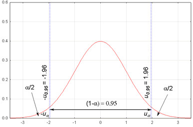
where x̄ is the sample mean, Z is the Z-value from the standard normal distribution corresponding to the desired confidence level (e.g., 1.96 for 95% confidence), and SE is the standard error of the mean.

Margin of Error

The margin of error reflects the maximum expected difference between the true population parameter and a sample estimate. It incorporates both the level of confidence and the variability in the data. The confidence level is commonly set at 95%, although other levels (like 90% or 99%) can also be used depending on the desired precision. The margin of error is calculated using the formula: Margin of Error = z or t * (SE)

Here:

• z or t: The z-score or t-score corresponding to the chosen confidence level

• SE: Standard error

Z-Scores and T-Scores

The selection between z-scores and t-scores depends on whether the population standard deviation is known and the sample size. For large sample sizes or when the population standard deviation is known, the z-score is used, which corresponds to the standard deviation in the standard normal distribution. Conversely, for smaller samples (n < 30) without the known population standard deviation, the t-score from the t-distribution is more appropriate, as it adjusts for the additional uncertainty.

The critical values (z or t) relevant to the most common confidence levels are:

• 1.96 for a 95% confidence interval using a z-distribution

• 2.58 for a 99% confidence interval using a z-distribution

• Values from the t-distribution table for a 95% or 99% confidence interval when using a t-distribution, varying based on degrees of freedom (df = n - 1)

Through these calculations, researchers can make informed estimates about population parameters, such as means or proportions, with a specified level of confidence.

Interpreting Confidence Intervals

When one interprets confidence intervals, it is critical to understand that they offer a range within which the true population parameter is estimated to lie, given a certain level of confidence. Confidence limits refer to the lower and upper bounds of a confidence interval, highlighting their role in framing the range within which the true population parameter is estimated to lie. This section will guide the reader through Interval Estimates and Confidence Levels to clarify their use in statistical analysis.

Interval Estimates

An interval estimate provides a range of values which, based on the sample data, is predicted to contain the population parameter like the mean or proportion. For example, a confidence interval for the mean of test scores might be presented as (100 pm 2.5) where 100 is the sample mean and 2.5 is the margin of error. The true mean of the population should be within this range.

Confidence Level

The confidence level signifies the frequency that the confidence interval, when computed from multiple samples, would contain the true population parameter. It is expressed as a percentage (e.g., 95% or 99%). A 95% confidence level suggests that if 100 different samples were taken and interval estimates computed, approximately 95 of those confidence intervals would contain the true population parameter.

Confidence interval calculation - examples

Confidence intervals are a fundamental statistical tool used across various fields to estimate the reliability of sample-based estimations. They offer a range within which one can expect, with a certain level of confidence, the true population parameter to lie.

Market Research - Product Pricing

A market research team wants to determine the ideal pricing for a new coffee maker. They survey 150 potential customers and find that the average willingness to pay is $120 with a standard deviation of $20.

Calculation:

• Sample Mean (ˉxˉ): $120

• Standard Deviation (s): $20

• Sample Size (n): 150

• Standard Error (SE):

  

• Z-value for 95% confidence: 1.96 (normal distribution used due to large sample size)

95% Confidence Interval:

CI=xˉ±(Z×SE)=120±(1.96×1.633)

CI=120±3.2

CI=[116.8,123.2]

This interval suggests that the company can be 95% confident that the true average willingness to pay for the coffee maker among all potential customers is between $116.80 and $123.20.

Marketing Research - Advertising Effectiveness

A marketing team runs an online advertising campaign and wants to estimate the increase in brand awareness. They sample 100 viewers and find an increase of 15 percentage points in brand awareness, with a standard deviation of 8 percentage points.

Calculation:

• Sample Mean (x̄): 15%

• Standard Deviation (s): 8%

• Sample Size (n): 100

• Standard Error (SE):

  

• Z-value for 95% confidence: 1.96

95% Confidence Interval:

CI=xˉ±(Z×SE)=15±(1.96×0.8)

CI=15±1.568

CI=[13.432,16.568]

This shows that the marketing team can be 95% confident that the true increase in brand awareness due to the advertising lies between 13.432% and 16.568%.

Example 3: UX Research - Website Usability Improvement

A UX team measures the time it takes users to complete a specific task on a website before and after a redesign. The average improvement in task completion time among 40 users is 30 seconds, with a standard deviation of 10 seconds.

Calculation:

• Sample Mean (x̄): 30 seconds

• Standard Deviation (s): 10 seconds

• Sample Size (n): 40

• Standard Error (SE):

  

• t-value for 95% confidence with 39 degrees of freedom: approximately 2.02 (from t-distribution table)

95% Confidence Interval:

CI=xˉ±(t×SE)=30±(2.02×1.58)

CI=30±3.1916

CI=[26.8084,33.1916]

This confidence interval indicates that the UX team can be 95% confident that the true average improvement in task completion time due to the website redesign is between 26.8084 seconds and 33.1916 seconds.

Statistical Comparison Between Two Slogans

Let's consider a marketing example where a company is testing two different advertising slogans to determine which one resonates more effectively with its audience. The company will measure the impact of these slogans on consumer purchase intent through a survey.

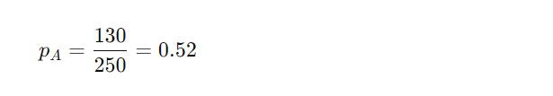
• Slogan A: Tested on 250 consumers, 130 indicated it increased their purchase intent.

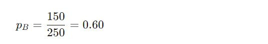
• Slogan B: Tested on 250 consumers, 150 indicated it increased their purchase intent.

Determine if there is a statistically significant difference in the effectiveness of the two slogans based on consumer responses.

• Slogan A: 130 out of 250 consumers responded positively.

• Slogan B: 150 out of 250 consumers responded positively.

Calculation:

Proportions

• Slogan A

• Slogan B

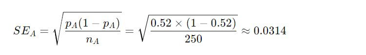
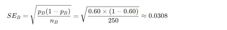
Standard Error of the proportion for each slogan:

• Slogan A

• Slogan B

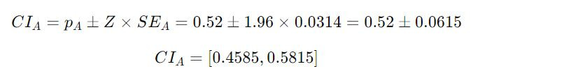
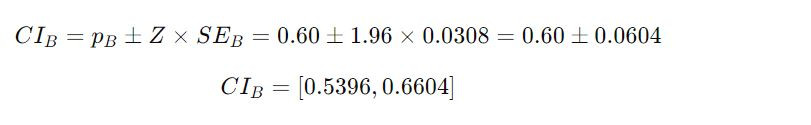
95% Confidence Interval for each slogan (using Z-value of 1.96 for 95% confidence):

• Slogan A

• Slogan B

Analysis:

• Slogan A's Confidence Interval: 0.4585 to 0.5815

• Slogan B's Confidence Interval: 0.5396 to 0.6604

The confidence intervals for Slogan A (0.4585 to 0.5815) and Slogan B (0.5396 to 0.6604) overlap. Therefore, the difference between the two slogans in terms of increasing purchase intent is not statistically significant. This overlap indicates that the data does not provide strong evidence to favor one slogan over the other based on the surveyed sample.

This detailed example demonstrates how confidence intervals can be used in customer surveys to statistically evaluate the significance of differences in proportions, offering clear insights into customer preferences.

Types of Confidence Intervals

Confidence intervals come in various forms to accommodate different statistical situations. They are essential tools in inferential statistics, providing a range within which one can expect to find a population parameter with a certain degree of confidence. The 'upper limit' of a confidence interval is crucial in determining the highest value within the range that is likely to contain the population parameter, playing a pivotal role in statistical calculations for parameters like σ2 or the population mean, as well as in determining ranges for relative risk and odds ratio.

One-Sample Interval

A one-sample confidence interval is used when one wants to estimate the population parameter based on a single sample. Typically, it's applied to estimate the mean or proportion when there is just one group under examination. For example, if a study aims to estimate the average height of adult women in a city, researchers would use the data from a single random sample of women to construct the interval.

Two-Sample Interval

Conversely, a two-sample confidence interval compares the difference between two independent groups. This kind of confidence interval is especially useful when the goal is to compare the means from two distinct groups. For example, comparing the average systolic blood pressure between smokers and non-smokers involves estimating the difference of the means from two separate samples, leading to a two-sample confidence interval.

Confidence Interval vs. Hypothesis Testing

Understanding the distinction between a confidence interval and hypothesis testing is essential for interpreting statistical results accurately. Both methods offer different insights about population parameters based on sample data.

Comparison

A confidence interval provides a range of values within which researchers can say with a particular level of certainty that a population parameter lies. For instance, a 95% confidence interval for a population mean tells us that, if the same population is sampled numerous times and intervals calculated, about 95% of them would contain the true population mean.

On the other hand, hypothesis testing is used to assess the evidence against a null hypothesis, a default statement that no effect or difference exists. This test yields a p-value, which indicates the probability of observing the sample data, or something more extreme, under the presumption that the null hypothesis is true.

When to Use Each Method

Researchers use a confidence interval when they are interested in estimating the range within which a population parameter falls. It is beneficial for understanding the precision of the estimate and the degree of uncertainty associated with it.

Hypothesis testing is more appropriate when researchers aim to make a decision or test a specific claim about a population parameter. They may want to determine whether the observed sample data provides enough evidence to reject the null hypothesis or not.

Both methods are integral to the field of inferential statistics, yet they serve different purposes and provide different kinds of information. A clear grasp of when and how to employ these techniques is crucial for conducting robust statistical analyses.

Challenges in Constructing Confidence Intervals

Constructing confidence intervals involves precise calculations and considerations. Notwithstanding the theoretical clarity, practitioners may confront several challenges, particularly when dealing with non-normal data distributions and handling small sample sizes.

Non-Normal Data

When data does not follow a normal distribution, establishing a confidence interval becomes more complex. Traditional methods for confidence interval construction often hinge on the assumption that the data conforms to normality. If this assumption is violated, the resulting interval may be inaccurate. For instance, with skewed data, especially if it's heavily skewed, the usual parameters for calculating intervals, like the mean and standard deviation, might not provide a true reflection of the data's central tendency and variability.

Scholars have developed alternative techniques to tackle such scenarios, including the application of non-parametric methods. These methods are not reliant on the data being normally distributed, often involving techniques like bootstrapping where samples are repetitively drawn from the data set with replacement to form a distribution of the estimate.

Small Sample Sizes

Small sample sizes present another challenge in the accurate calculation of confidence intervals. With a limited number of observations, the central limit theorem does not apply robustly, which asserts that given a sufficiently large sample size, the sampling distribution of the mean will be normally distributed. In such cases, the usual ( z )-score that is employed in constructing confidence intervals for large samples becomes unreliable and might lead to intervals that do not capture the population parameter effectively.

Addressing small sample sizes frequently involves the use of the ( t )-distribution, which adjusts for the increased variability inherent in smaller samples. The degrees of freedom, linked to the sample size, become crucial in determining the appropriate ( t )-values to use. This can be more efficient than the normal approximation in providing a more reliable estimation of the confidence intervals for small sample sizes.

Frequently Asked Questions

This section addresses common queries surrounding the concept and utilisation of confidence intervals in statistical analysis.

What constitutes a confidence interval in statistical analysis?

A confidence interval in statistical analysis is a range of values that is likely to contain the true value of a population parameter. It provides an estimate of the degree of uncertainty associated with a sample statistic.

How is a 95% confidence interval calculated and interpreted?

A 95% confidence interval is calculated using the standard error of the mean and a critical value from the distribution that corresponds to the desired confidence level. To interpret this interval, one would say that with 95% confidence, the true population parameter lies within this range.

In what ways are confidence intervals applied in practical situations?

Confidence intervals are applied in various practical situations such as in medical research to estimate the effectiveness of a drug, in quality testing to determine product reliability, or in survey research to assess public opinion with a known margin of error.

What are three common confidence levels used in statistical significance tests?

Three common confidence levels used in statistical significance tests include 90%, 95%, and 99%. These levels of confidence correspond to the probability that the true parameter exists within the calculated interval.

What is the meaning behind the term 'confidence level' in the context of statistical inference?

The term 'confidence level' in the context of statistical inference quantifies the probability that the calculated confidence interval actually contains the true population parameter. This level reflects the frequency with which an interval would capture the parameter if the same study were repeated multiple times under the same conditions.